Use trends in forecasting
When you choose to generate a forecast with trends, WFM calculates an annual growth rate in contact volume.
The choice of reference periods is an art that should take into account any seasonal fluctuations in the historical data. If historical data is seasonal, it is best to use the same portions of two different years to determine the trend.:
Calabrio ONE uses linear trends for forecasting. You can use two different trend options to generate a forecast:
- Historical trend—WFM uses historical data from your chosen reference period to calculate the percentage of contact volume change for each day of the week that is then applied to every date in the forecast period.
- Expected trend—WFM uses the annual growth rate you supply to calculate the contact volume change for every date in the forecast period.
Historical trends
Standard forecasting method
This trend option uses two reference periods. For each of the two trend reference periods, the average contact volume for each day of the week is computed, as well as the median date for each day of the week. For example, if there are five instances of Wednesday in the reference period, the median Wednesday is the third instance of that day.
Additionally, for each reference period, an overall average contact volume and mean date are computed. Then, the results from the two reference periods are combined to produce a growth rate and growth duration. From this, the annual growth rate is computed.
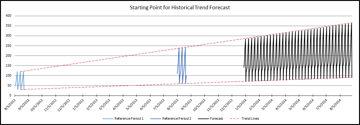
In a forecast using a historical trend, the starting point of the forecast is calculated by extending the trend line from the midpoint of the second reference period to the beginning of the forecast. In the graph below, the two reference periods are one year apart and there has been 100 percent growth over the course of the year (true for all days of the week). This growth is extended until January of the following year when the forecast begins.
Advanced forecasting method
This trend option uses two reference periods. For each of the two trend reference periods, the average contact volume for each day of the week is computed, as well as the median date for the reference period. For example, if there are five instances of Wednesday in the reference period, the median Wednesday is the third instance of that day.
Once the overall average contact volume and mean date are computed for each reference period, these values are used to produce a difference in contact volume and difference in time. The annual growth rate is computed from this.
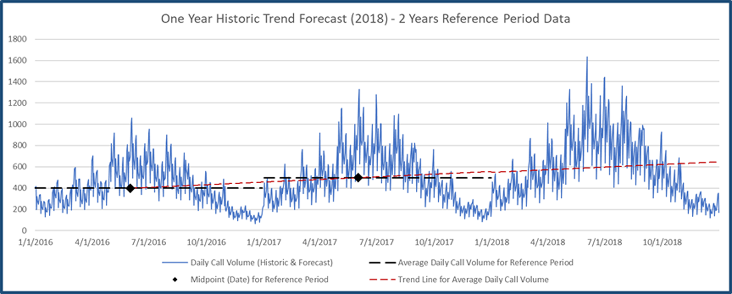
In a forecast using a historical trend, the starting point of the forecast is calculated by extending the trend line from the midpoint in the second reference period to the beginning of the forecast. In the graph below, the two reference periods are one year apart and there has been 100 percent growth over the course of the year. This growth is extended until January of the following year when the forecast begins.
Expected trends
Standard forecasting method
In a forecast using a user-supplied expected trend, you enter a single reference period and a percentage rate of annual growth. A simple example is an annual growth rate of 100 percent. After one full year, call volume will have doubled (increased by 100 percent). The rate of growth is the same for all days of the week, but the slope of the linear trend associated with each day of the week might be different (see the Day of the week effect).
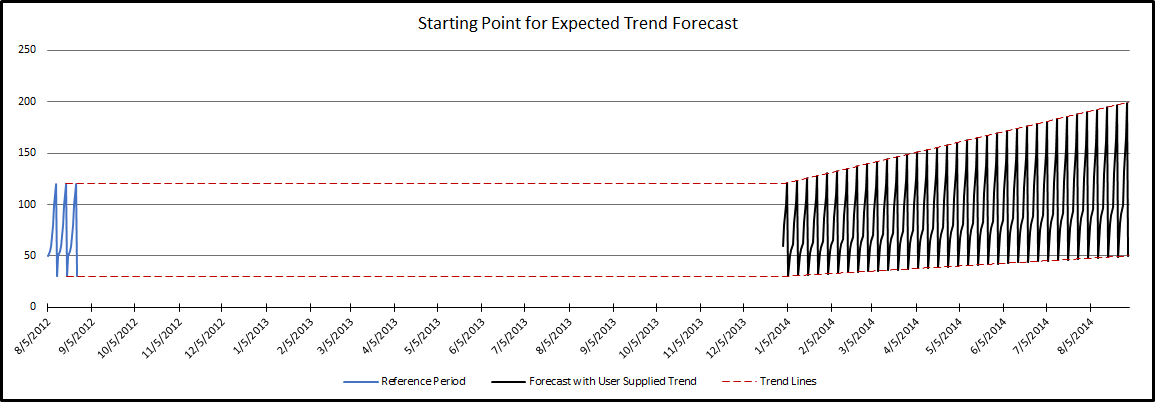
The average call volume is calculated on a per-day-of-the-week basis and carried forward to the first day of the forecast. It does not matter how much time elapses between the reference period and the beginning of the forecast (see the chart below). If the forecast begins on the same day of the week, the starting values will be identical between forecasts. If it begins on a different day of the week, there will be a small margin of error since the trend is applied to each forecast date.
Advanced forecasting method
In a forecast using a user-supplied expected trend, you enter a single reference period and a percentage rate of annual growth. A simple example is an annual growth rate of 100 percent. After one full year, the average daily call volume will have doubled (increased by 100 percent).
The average daily call volume is calculated from the whole reference period and carried forward to the first day of the forecast. It does not matter how much time elapses between the reference period and the beginning of the forecast (see the chart below). Since there are seasonal factors involved, the beginning forecast value will only be very close to the beginning reference period value if the forecast starts on the same day of the week, month of the year, and day of the month.
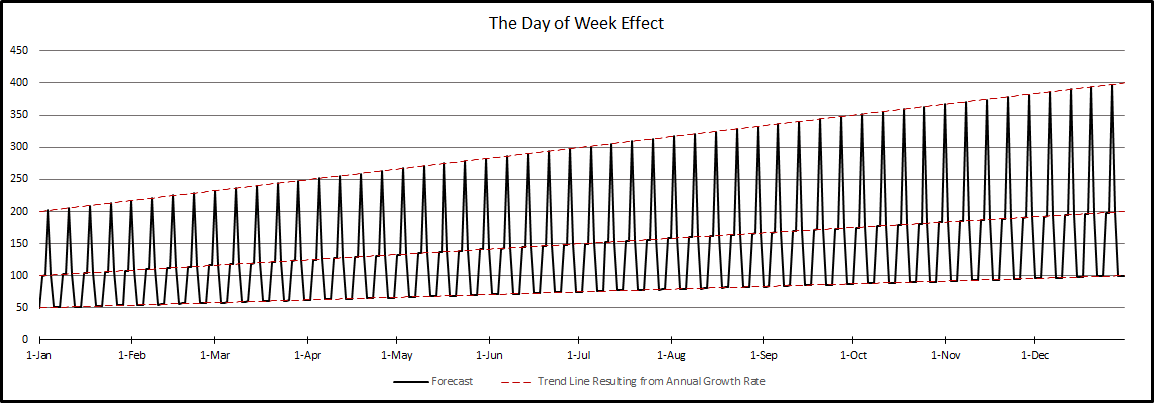
Day of the week effect
Since different days of the week usually have different call volumes, the effect of a uniform annual growth rate differs by day of the week. In the example below, the annual growth rate is 100 percent. The starting and ending average call volume for each day of the week is displayed in the following table:
| Day of the Week | Initial Call Volume | Call Volume After 1 Year |
|---|---|---|
| Sunday | 50 | 100 |
| Monday | 50 | 100 |
| Tuesday | 50 | 100 |
| Wednesday | 100 | 200 |
| Thursday | 100 | 200 |
| Friday | 200 | 400 |
| Saturday | 100 | 200 |
The red dashed lines show the trend line that results from the growth rate.
Examples: One-year forecast using the standard forecasting method
This section contains examples of the expected behavior of year-long forecasts made with specific growth rates. The annual growth rate is the amount of expected growth seen one full year after the beginning of the forecast.
NOTE The formula uses 365 days in regular years and 366 days in leap years as the year length. In a normal year, the amount of growth on the 365th day of the forecast affecting the average call volume used to forecast will equal the average plus the expected growth.
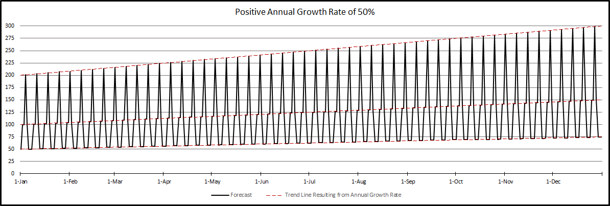
Example 1: Positive growth rate
In this example, the annual growth rate is 50 percent. At the end of one year, the call volume for each day of the week should increase to 1.5 times its original value.
| Day of the Week | Initial Call Volume | Call Volume After 1 Year |
|---|---|---|
| Sunday | 50 | 75 |
| Monday | 50 | 75 |
| Tuesday | 50 | 75 |
| Wednesday | 100 | 150 |
| Thursday | 100 | 150 |
| Friday | 200 | 300 |
| Saturday | 100 | 150 |
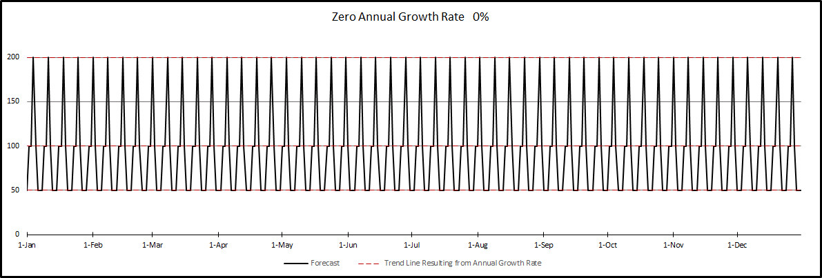
Example 2: Zero growth rate
In this example, there is no change to the call volumes by day of the week (an annual growth rate of zero percent). The forecast for each day of the week is perfectly flat.
| Day of the Week | Initial Call Volume | Call Volume After 1 Year |
|---|---|---|
| Sunday | 50 | 50 |
| Monday | 50 | 50 |
| Tuesday | 50 | 50 |
| Wednesday | 100 | 100 |
| Thursday | 100 | 100 |
| Friday | 200 | 200 |
| Saturday | 100 | 100 |
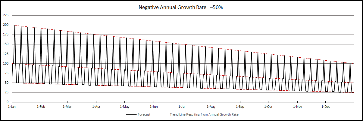
Example 3: Negative growth rate
In this example, the call volume is decreasing. In the first chart, an annual growth rate of –50 percent implies that the call volumes for each day of the week is half of their starting value after one year.
| Day of the Week | Initial Call Volume | Call Volume After 1 Year |
|---|---|---|
| Sunday | 50 | 25 |
| Monday | 50 | 25 |
| Tuesday | 50 | 25 |
| Wednesday | 100 | 50 |
| Thursday | 100 | 50 |
| Friday | 200 | 100 |
| Saturday | 100 | 50 |
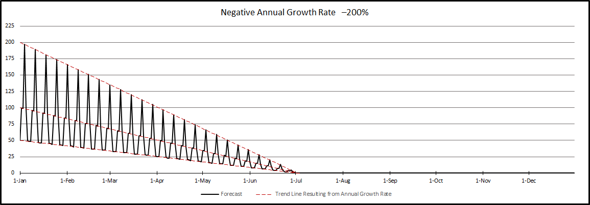
In the second chart, the annual growth rate is –200 percent. In this case, the call volumes reach zero halfway through the year. Once a negative growth rate forces the forecast to converge to zero, it bottoms out and can never be less than that. Because of the day of the week effect (see Day of the week effect), all days of the week converge to zero at roughly the same point in time.
Examples: One-year forecast using the advanced forecasting method
This section contains examples of the expected behavior of year-long forecasts made with specific growth rates. The annual growth rate is the amount of expected growth seen one full year after the beginning of the forecast.
NOTE The formula uses 365 days in regular years and 366 in leap years as the year length. The amount of growth on the 365th day of the forecast will not be exactly equal to the annual growth rate, but it should be very close and within an acceptable margin of error.
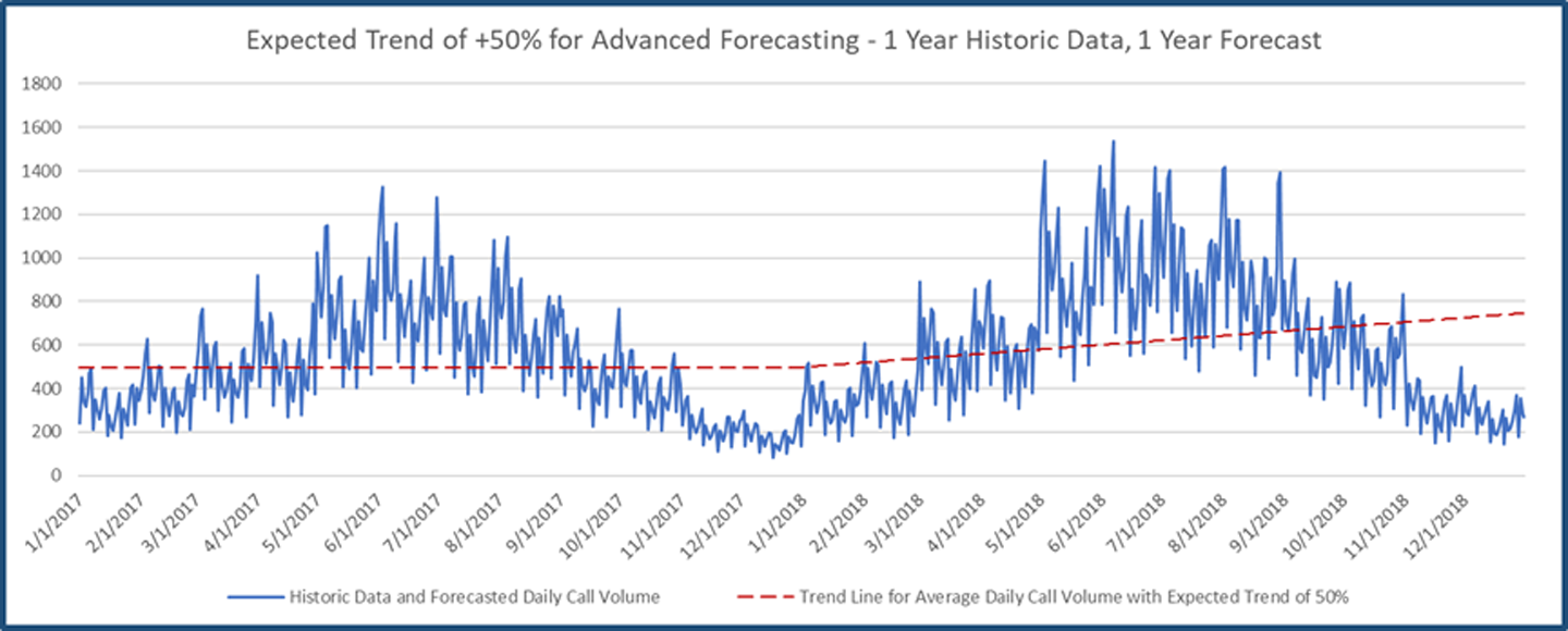
Example 1: Positive growth rate
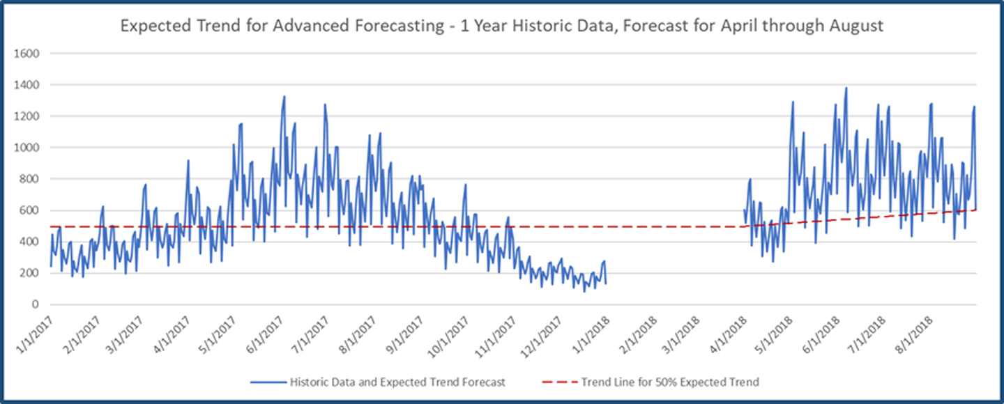
In this example, the annual growth rate is 50 percent. The average call volume increases so that at the end of one year, the average call volume will have increased to 1.5 times its original value. In the table and graph below, the average call volume begins at 497.7 and increases to 745.7 after one year. The average call volume for the last day of each month is shown in the table.
| Month | Reference Period Average Daily Call Volume | Average Call Volume at End of the Month |
|---|---|---|
| January | 497.7 | 518.1 |
| February | 497.7 | 537.2 |
| March | 497.7 | 558.3 |
| April | 497.7 | 578.8 |
| May | 497.7 | 599.9 |
| June | 497.7 | 620.3 |
| July | 497.7 | 641.5 |
| August | 497.7 | 662.6 |
| September | 497.7 |
683.0 |
| October | 497.7 | 704.1 |
| November | 497.7 | 724.6 |
| December | 497.7 | 745.7 |
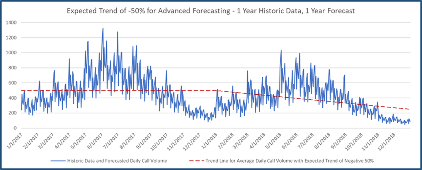
Example 2: Negative growth rate
In this example, the call volume is decreasing. In the first table and graph, an annual growth rate of –50 percent is applied so that the average daily call volume after one year is half of what it is at the beginning of the forecast period. In the table below, the average daily call for each month is shown.
| Month | Reference Period Average Daily Call Volume | Average Call Voilume at End of the Month |
|---|---|---|
| January | 497.7 | 477.3 |
| February | 497.7 | 458.2 |
| March | 497.7 | 437.1 |
| April | 497.7 | 416.6 |
| May | 497.7 | 395.5 |
| June | 497.7 | 375.1 |
| July | 497.7 | 353.9 |
| August | 497.7 | 332.8 |
| September | 497.7 | 312.4 |
| October | 497.7 | 291.3 |
| November | 497.7 | 270.8 |
| December | 497.7 | 249.7 |
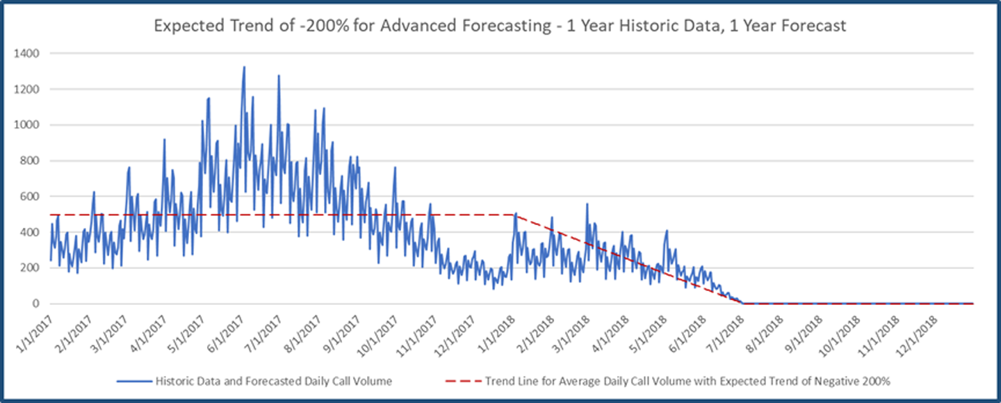
In the second chart, the annual growth rate is –200 percent. In this case, the call volumes reach zero halfway through the year. Once a negative growth rate forces the forecast to converge to zero, it bottoms out and can never be less than that. Due to Day of Week arrival patterns, not all days may reach zero at the same point in time, as seen in the graph.
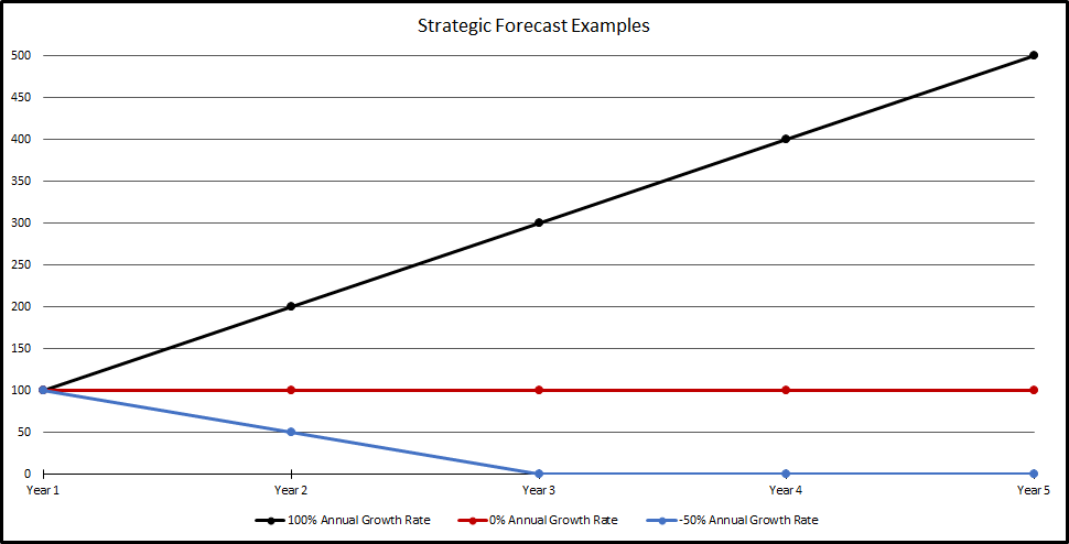
Strategic forecasts
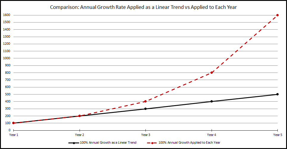
Strategic forecasts are 5 years long. The annual growth rate is used to calculate the expected growth at the one-year point in time and to calculate the slope of the line that describes the call volume’s continued growth. This is shown in the graph below as an annual growth rate as a linear trend. The growth rate is not applied independently to each year of the strategic forecast. The dashed red line illustrates what happens when the growth rate is applied to each subsequent year of a forecast.
Strategic forecast examples
Below are some examples of an annual growth rate as a linear trend (expected trend) in a strategic forecast. The annual growth rates shown are 100 percent, zero percent, and –50 percent. In all examples, the starting point is the same. Notice that a growth rate of –50 percent over the first year reaches zero at the end of Year 2, and then remains there for the rest of the forecast. Also worth noting is the zero percent growth rate (there is no change in the call volume for the forecast).